Second Distribution Transformer Analysis

We have analyzed 26 distribution transformers in DC, Maryland, Virginia, Iowa, Helsinki, and New Hampshire. This analysis builds on the foundation set in the initial distribution transformer analysis; of most relevance is the section "What are we looking for?", and the separate overview that discusses the physical phenomena behind a transformer's acoustics.

The observations below of distribution transformers show that.

Selecting the Right Fourier

Fourier transforms combine many different parameters, and selecting them for the situation is a form of art. Fourier transforms are primarily categorized by the frame size (how many samples we're looking at). While padding zeros in the data allows for greater precision when determining the underlying frequencies (since it increases the frame size), it does not offer greater accuracy — the same result could be determined through interpolation.

Frame Size (Fourier Frequency)

The Fourier transform is subject to a basic tradeoff that is similar to the Heisenberg uncertainty principle (in German, "the unsharpness relation") which says that you can know when something happened or what something was, but not both. In this context, as we increase the accuracy of the frequency, we decrease the accuracy of the time.

Knowing this, we can look at a pole-mounted transformer hoisted 20 feet in the air. There was considerable background noise at the time from local landscaping equipment. This recording was made at a 44.1 kHz sampling rate. If we supply 44,100 data samples (one second's worth of data — performing a Fourier transform at a rate of 1 Hz), we have a hard time making out the 120 Hz tone that is characteristic of transformers.

 

Given that our Fourier transforms have smaller frame sizes, we can make more sense of a longer period of time. The Y-axis is time, the X-axis is frequency, and the color is the relative volume in decibels (relative to the loudest noise). We are able to make out the loud activity of the landscaping equipment and can see every time the spinning blades slow down when they cut through brush.

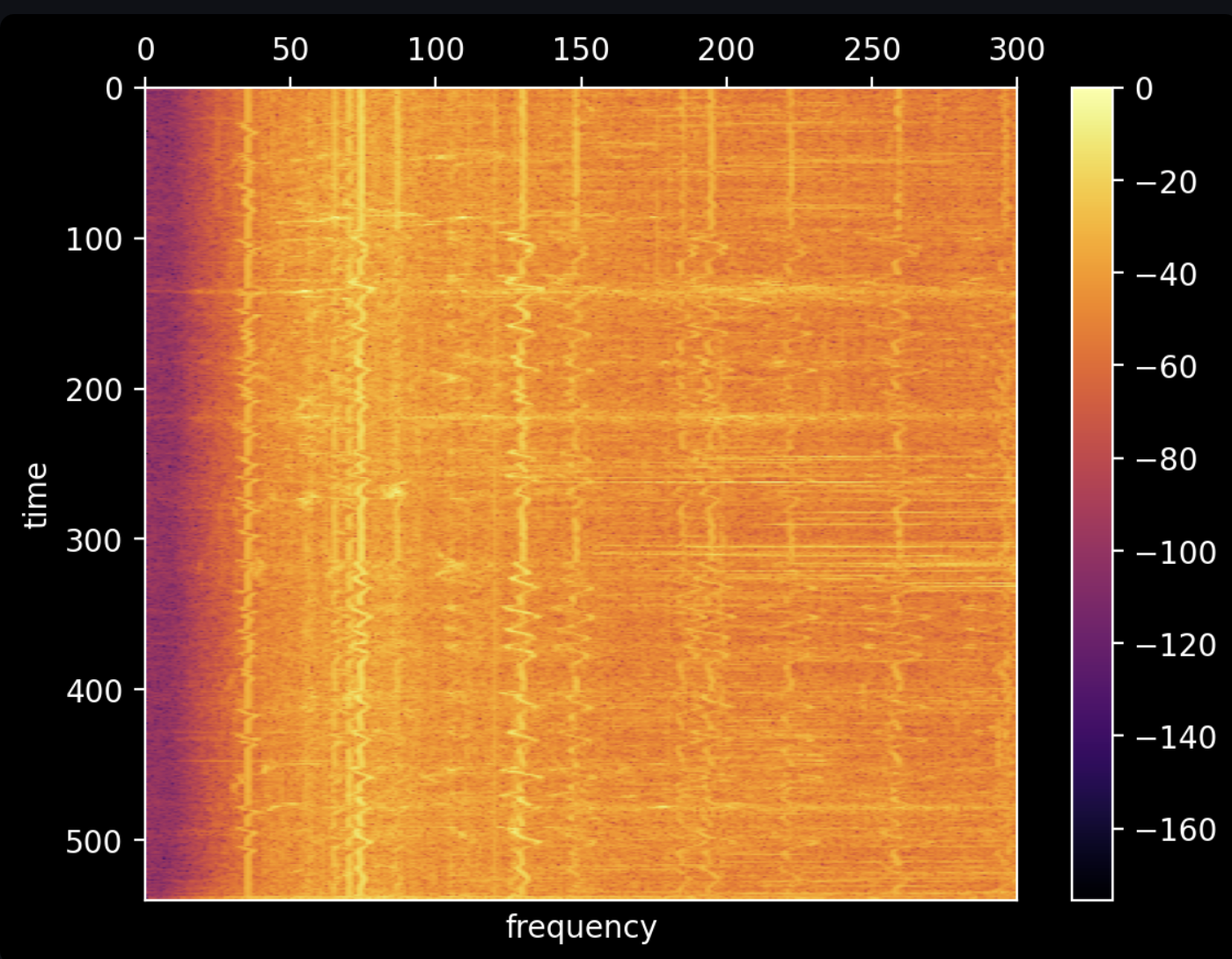
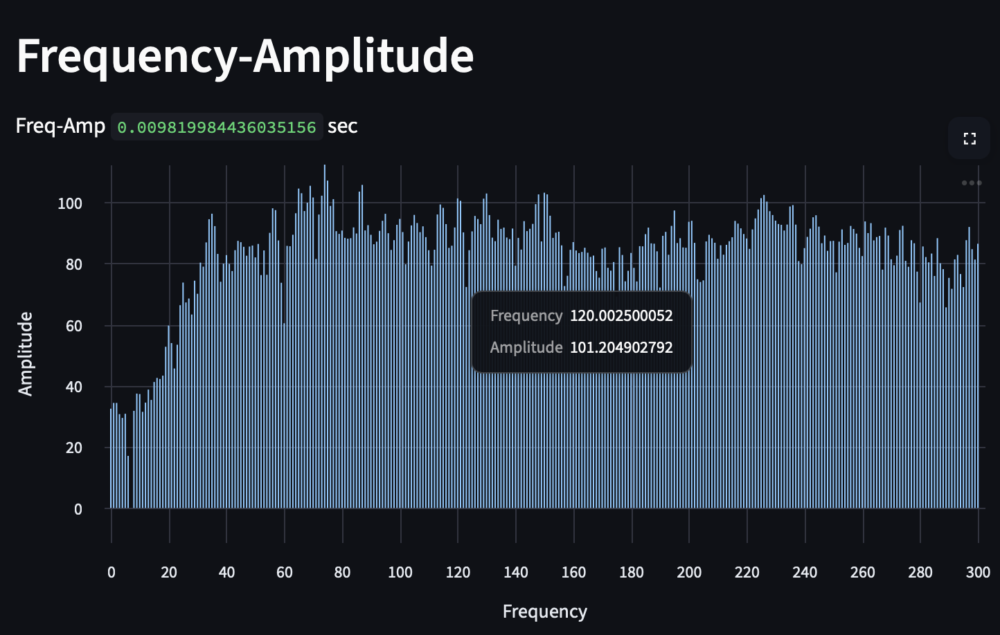
There is a subtle line marking 120 Hz, but it's tough to get anything useful out of it. We can increase the frame size to increase the accuracy and precision of the frequencies in the data. In the below graph, we decrease the frequency of our Fourier transforms to be one every 100 seconds, increasing the frame size to 4,410,000 samples. As you can see below, we sacrifice our ability to detect when something is happening:

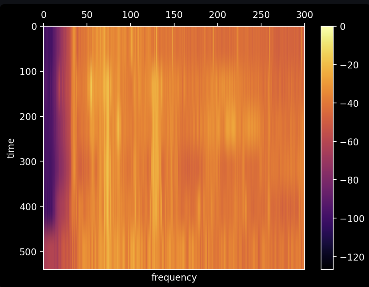
But we gain the ability to see what we're listening to (this is the Fourier transform of the first 100 seconds):

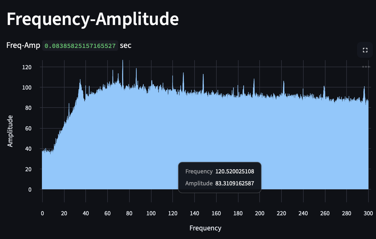
In the above graph, we can see quite clearly that there is a strong 120 Hz tone. The wide peaks mean that the frequency was wavering over the time period of the frame, and the sharp peak of the 120 Hz tone implies stability.