Second Distribution Transformer Analysis

We have analyzed 26 distribution transformers in DC, Maryland, Virginia, Iowa, Helsinki, and New Hampshire. This analysis builds on the foundation set in the initial distribution transformer analysis; of most relevance is the section "What are we looking for?", and the separate overview that discusses the physical phenomena behind a transformer's acoustics.

The observations below of distribution transformers show that.

Power Quality Analysis from Acoustics

asdf

Transformer Load Estimation from Acoustics

One recent breakthrough was the discovery of an IEEE paper "Load Estimation for Transformer Based on Acoustic Features" (2025), which declared that we could do more than just assess a transformer's health — we could estimate the transformer loading. In addition, their technique uses the same recording devices and the same feature (approximately the total harmonic distortion [THD] of the 120 Hz fundamental frequency). The researchers used a linear regression, but Bellwether's further assessment finds that the loading-THD relation conforms to a logarithmic regression better than a linear regression.

Next Step

As of November 2025, we are unable to reproduce the paper's findings because we do not have the requisite transformer loading data that is required. However, we are looking to partner with a utility in order to acquire that data, reproduce the paper's findings, and develop a non-invasive, passive, handheld tool to allow for relevant parties to assess the loading of a transformer.

Selecting the Right Fourier

Fourier transforms combine many different parameters, and selecting them for the situation is a form of art. Fourier transforms are primarily categorized by the frame size (how many samples we're looking at). While padding zeros in the data allows for greater precision when determining the underlying frequencies (since it increases the frame size), it does not offer greater accuracy — the same result could be determined through interpolation.

Frame Size (Fourier Frequency)

The Fourier transform is subject to a basic tradeoff that is similar to the Heisenberg uncertainty principle (in German, "the unsharpness relation") which says that you can know when something happened or what something was, but not both. In this context, as we increase the accuracy of the frequency, we decrease the accuracy of the time.

Knowing this, we can look at a pole-mounted transformer hoisted 20 feet in the air. There was considerable background noise at the time from local landscaping equipment. This recording was made at a 44.1 kHz sampling rate. If we supply 44,100 data samples (one second's worth of data — performing a Fourier transform at a rate of 1 Hz), we have a hard time making out the 120 Hz tone that is characteristic of transformers.

Parameter	Value
Sampling Rate	44.1 kHz
Frame Duration	1 second
Frequency Step	1 Hz

Given that our Fourier transforms have smaller frame sizes, we can make more sense of a longer period of time. The Y-axis is time, the X-axis is frequency, and the color is the relative volume in decibels (relative to the loudest noise). We are able to make out the loud activity of the landscaping equipment and can see every time the spinning blades slow down when they cut through brush.

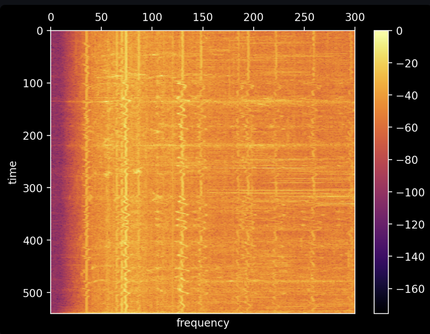
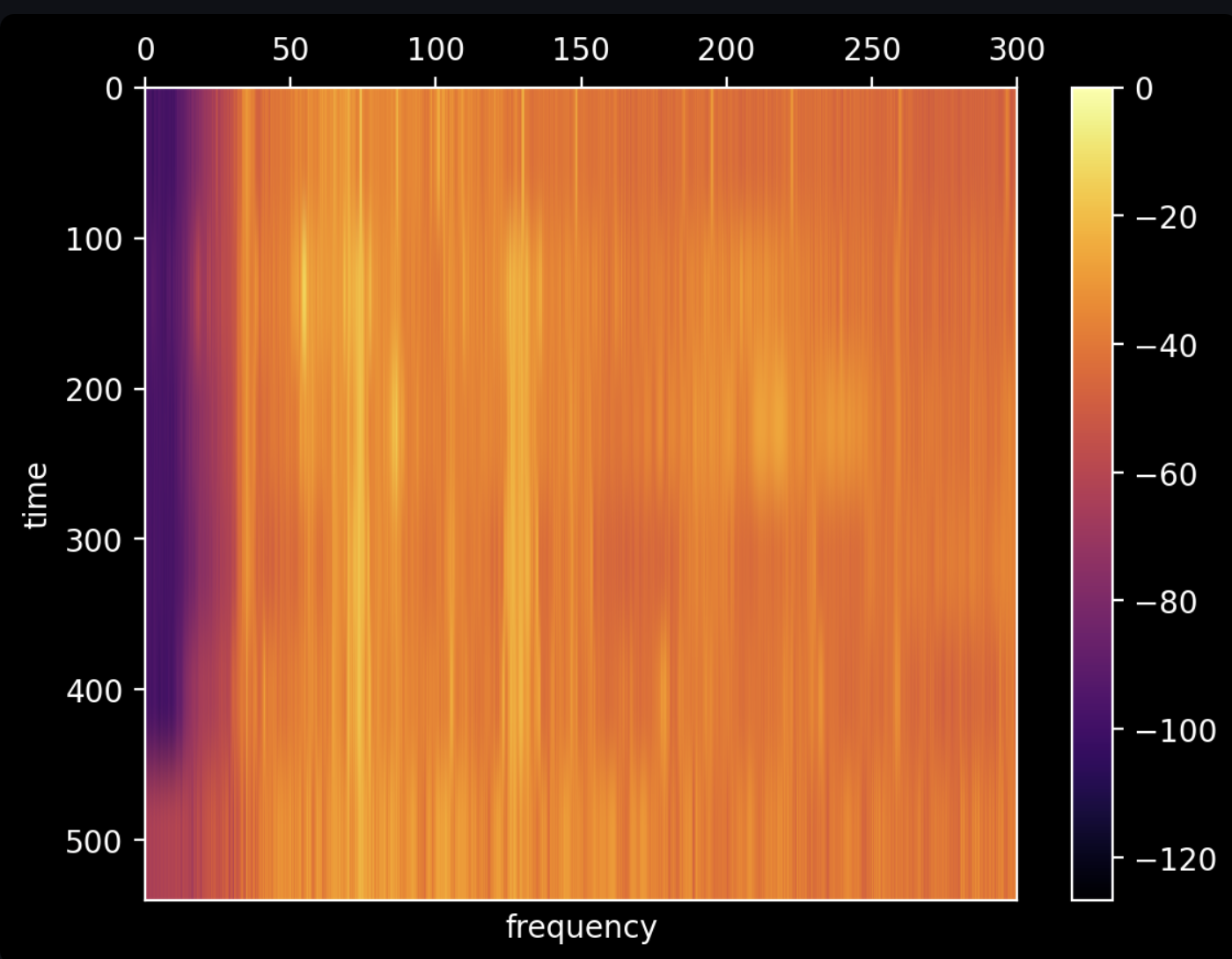
There is a subtle line marking 120 Hz, but it's tough to get anything useful out of it. We can increase the frame size to increase the accuracy and precision of the frequencies in the data. In the below graph, we decrease the frequency of our Fourier transforms to be one every 100 seconds, increasing the frame size to 4,410,000 samples. As you can see below, we sacrifice our ability to detect when something is happening:

Parameter	Value
Sampling Rate	44.1 kHz
Frame Duration	100 seconds
Frequency Step	0.01 Hz

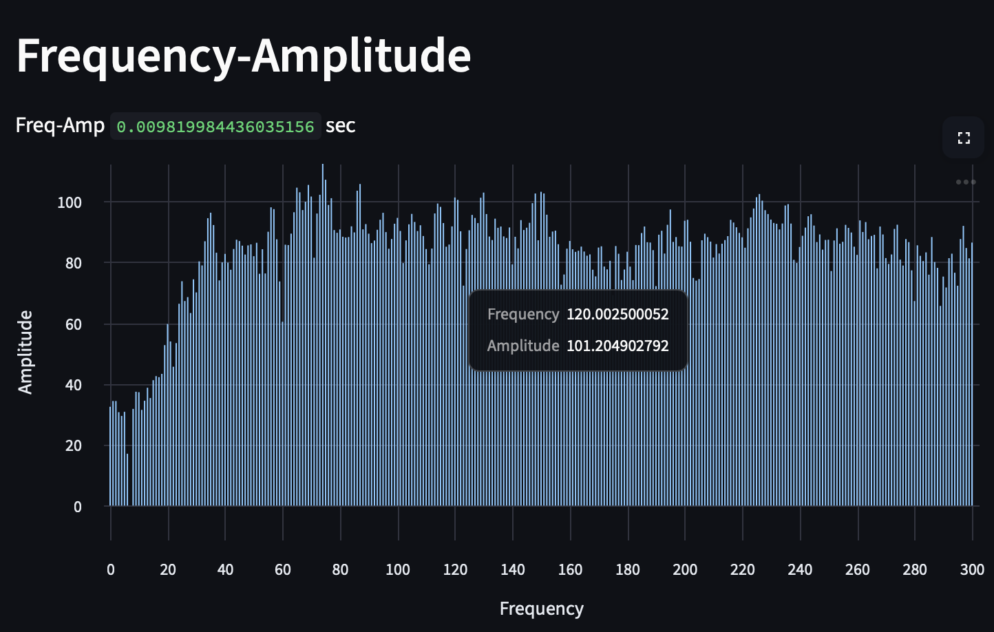
But we gain the ability to see what we're listening to (this is the Fourier transform of the first 100 seconds):

In the above graph, we can see quite clearly that there is a strong 120 Hz tone. The wide peaks mean that the frequency was wavering over the time period of the frame, and the sharp peak of the 120 Hz tone implies stability.

This serves as a single example demonstrating how to effectively extract a signal that is otherwise hidden among the noise, and it is the primary tool for combatting loud environments and interfering noise.

Harmonic Deviation — Harmonics vs Noise

Parameter	Value
Sampling Rate	44.1 kHz
Frame Duration	100 seconds
Frequency Step	0.01 Hz

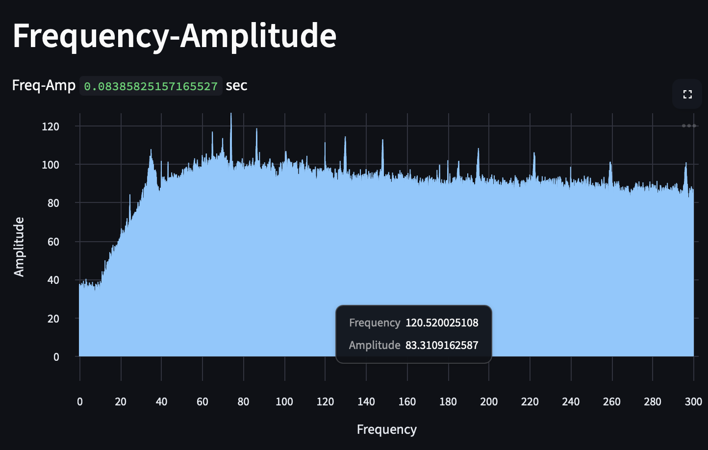
Previously, we looked at the relative strength of a harmonic, asking how many standard deviations above the mean a given frequency was above the mean of its surrounding frequencies. An example distribution of a Virginia substation is below. It was recorded from the grass 20 feet from the fence, which is another 40 feet from the transformers.

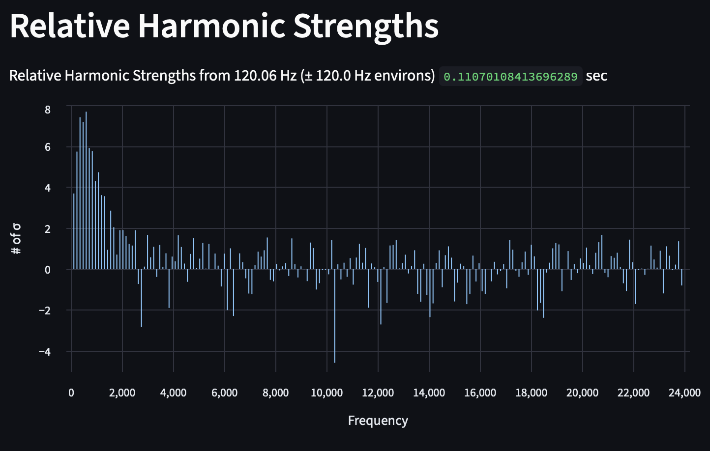
Our next question introduces a new analytical technique, asking whether these frequencies are actual peaks.

1. We start with a fundamental frequency that is determined by finding the peak value within a given sideband of 120 Hz.
2. We then calculate the harmonics by multiplying the identified fundamental (e.g. 120.02 Hz) by the harmonic number (1, 2, 3, ...). This gives us a "calculated harmonic".
3. Then, we observe which frequency is the highest within a sideband (e.g. 0.5 Hz) of the calculated harmonic. This gives us our "actual harmonic".
4. We subtract the actual harmonic from the calculated harmonic to get the deviation.
5. The results are plotted.

Sideband of 0.25 Hz

With a sideband of 0.25 Hz, the substation's harmonic deviation starts out very small, but quickly grows after the 10th harmonic, where the deviations are larger but still grouped between -0.1 and 0.1. We can see another dispersal occur after the 35th harmonic, where it becomes truly random.

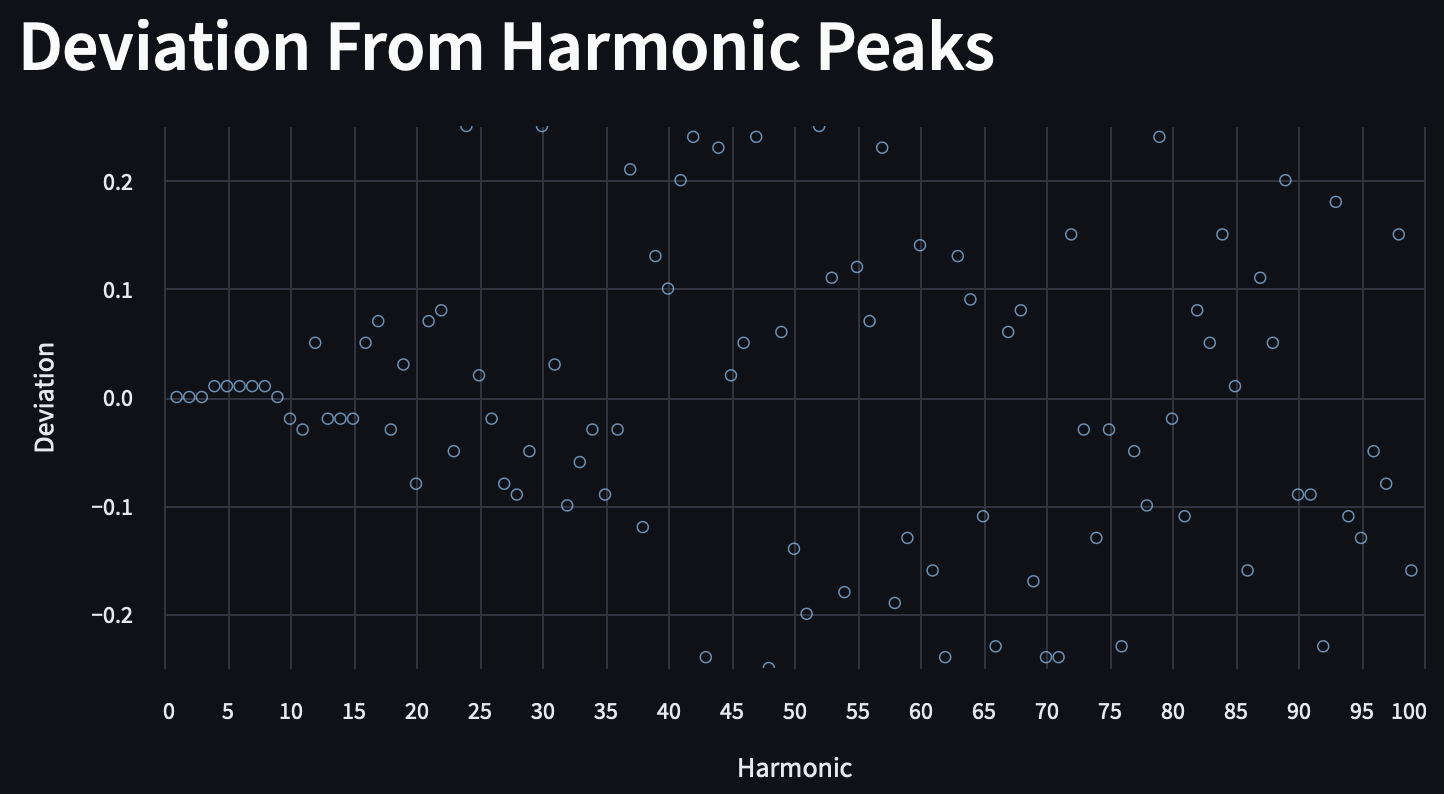
While this may suggest that the calculated peaks are no longer useful beyond the 10th harmonic, we have to consider the unknown margin of error in our instruments; expanding our sideband view offers a different perspective that clarifies reasonable deviation versus random noise. The presence of max and min values (0.25 and -0.25) of deviation here imply that we are stuck in troughs, and that the true peaks of harmonics > 40 lie outside of that restriction.

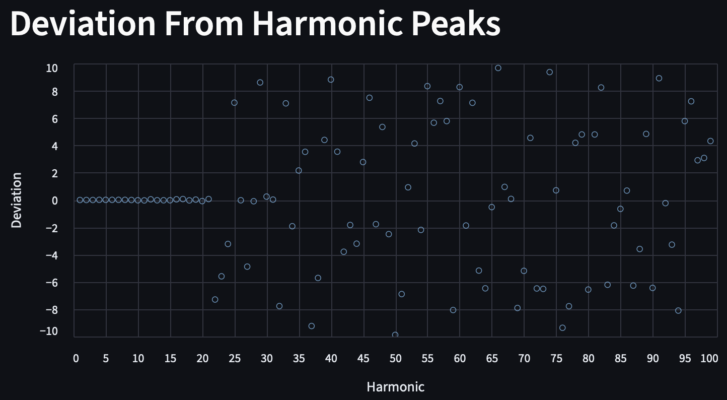
Sideband of 10 Hz

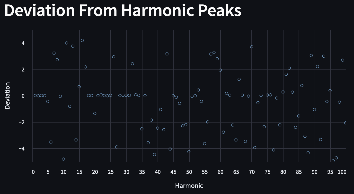
If we allow a 10 Hz sideband to find a peak frequency, we can see more encouraging results, which show strong and consistent harmonics that deviate very little from the calculated harmonics through the 21st harmonic.

Class Evaluation of Harmonic Deviation

Looking at the 26 transformers as a class, we can now measure how deep the harmonics go before beginning to significantly deviate, with a metric known as harmonic depth. Given the relationship between harmonics, distortion, and transformer overloading, we expect this metric to be useful in determining a transformer's loading.

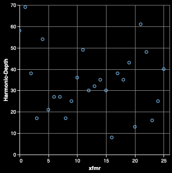
We can see that the harmonic depth of the transformers is evenly distributed across the range.

In the below plot of harmonic deviation (how much a calculated harmonic differs from the actual peak frequency within a 5 Hz band), we can see that there is nearly zero deviation up until the 4th harmonic. Then, some noise is introduced that obscures the transformer harmonics. Between the 18th and 36th harmonic, the intervening noise dissipates, and we are able to precisely identify the harmonic again. Noise variably intervenes from the 45th to the 76th harmonic.

When conducting any kind of further analysis on the harmonics, we take care to only use the harmonics that are within 0.5 Hz deviation, so that noise is not included.

Total Harmonic Distortion

Building off the work conducted by Zhao et al. (2025), we can assess what the THD of the transformers is. This is the metric they used to determine loading according to a linear regression. According to "Developing an Accurate Load Noise Formula for Power Transformers" (2019), the acoustic amplitude grows logarithmically as loading grows linearly, which would represent an innovation on top of Zhao's work to produce a more accurate estimation of transformer loading.

Harmonic Sequences

Harmonic sequences are defined as the positive, negative, and zero harmonics, which correspond to those whose harmonic number modulo 3 is 1, 2, and 0, respectively.

For a total of $m$ valid harmonics (whose deviation is less than 0.5 Hz from the detected nearby peak), the value is calculated as:

$\frac{\Sigma^m_n Amplitude_n^2}{Amplitude_1^2}$

The points are colored according to how many viable harmonics went into the calculation.

Positive Harmonics

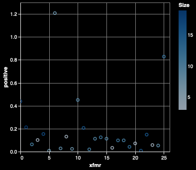
Positive harmonics cause the machinery to rotate forward greater than they should, and can cause excessive heating due to supplying more forward motion than is desired. This value is the ratio of the sum of the squares of the amplitudes of the positive harmonics to the square of the amplitude of the fundamental frequency (120 Hz).

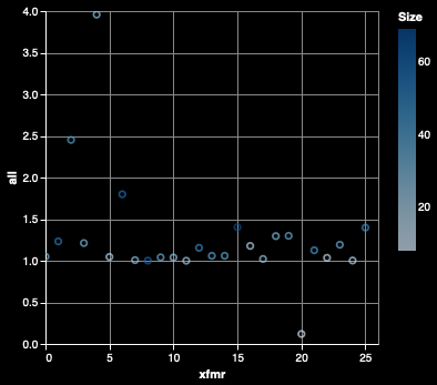
Transformer #6, the New Pioneer Food Coop transformer, in Iowa City, IA, stands out as an outlier with a positive-sequence THD of 1.2. Of note, it has an extremely weak fundamental frequency, which we will discuss later. This weak fundamental causes it to be an outlier in all metrics, so we will avoid any analysis on it for now. Below are the positive harmonic THDs for all transformers.

Below are the positive harmonics highlighted for a transformer in Baltimore, MD.

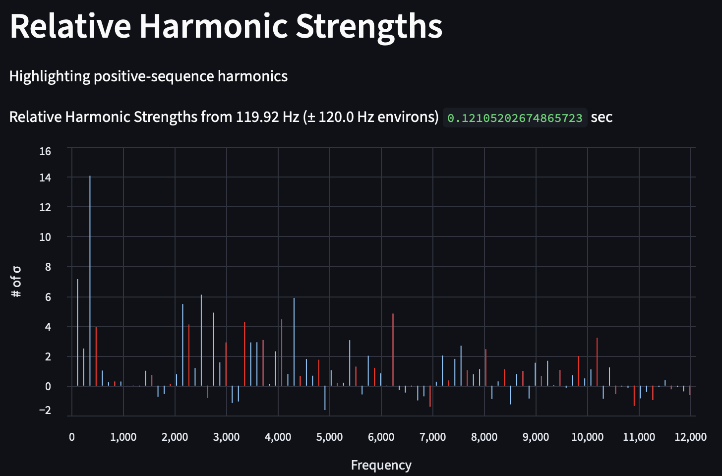
It's tough to draw any conclusions from this , but the strong 3rd harmonic calls our attention. Looking at this transformer when compared to the rest, we see that it is strong in all three sequences, but it is an outlier for both the positive- and zero-sequence harmonics:

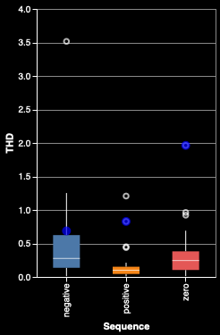
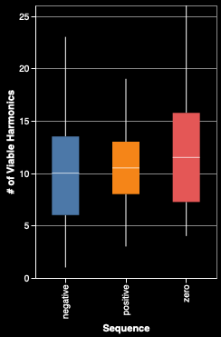
One thing this chart makes clear is that negative harmonics tend to be much rarer than the other types of harmonics. Looking at the spread of viable harmonics for each sequence (the table on the right), we can see that they are based on the same amount of harmonic information, which leads us to believe that the THD difference is meaningful.

This analysis will be enhanced by the introduction of loading data, with which we can correlate the harmonics to the loading.

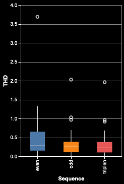
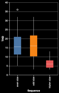
Harmonic Parity

The THD for the three parity metrics (even, odd, and triplen) all have roughly the same median values. Strangely, even harmonics have even greater THD, which is quite unexpected, as explained below. The graph on the left shows a box plot of the THD for each of the sequences. The graph on the right show the box plot for how many harmonics were used in the calculation of the THD.

Since odd and even harmonics are 1/2 of the available harmonics, and triplen are 1/6 (odd-numbered multiples of the 3rd harmonic), we can multiply each median by the denominator (2, 2, and 6) and verify that they're about the same, which means that they are equally represented in the data.

             

Even Harmonics

Within power quality analysis, even harmonics indicate DC biasing — theoretically, we shouldn't be seeing these on transformers. However, given that we're conducting acoustic analysis, and that there is likely a non-linear process of producing sound from the oscillating magnetic field, the rules are different; it is difficult to know what the even harmonics in the acoustic data mean.

Unusual Findings

Strong 120 Hz Fundamental

asdf

Weak 120 Hz Fundamental

New Pioneer Food Coop

Half Harmonics

asdf